Deconvolution Microscopy: Fundamentals, Applications, and Reproducible Results
A technical guide to deconvolution microscopy — what the point spread function is, how iterative algorithms recover lost signal, which modalities benefit most, and what it takes to get reproducible results across labs.
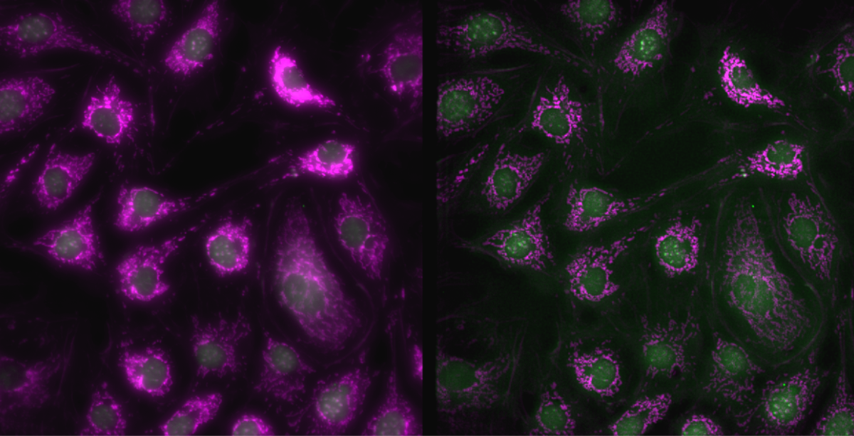
Deconvolution Microscopy: Fundamentals, Applications, and Reproducible Results
Fluorescence microscopy has transformed cell biology, neuroscience, and developmental biology over the past four decades. Yet every fluorescence image carries a hidden distortion: the point spread function (PSF). Deconvolution microscopy is the computational process of undoing that distortion — recovering the true spatial distribution of fluorophores from a blurred, noisy measurement.
This guide covers the physics behind image blur, the mathematics of deconvolution, the algorithms in common use, modality-specific considerations, and — critically — what it takes to produce results that are reproducible across instruments, operators, and institutions.
The Point Spread Function: Why Every Fluorescence Image Is Blurred
When a single fluorescent point source is imaged through an optical system, the detector does not record a point. It records a three-dimensional intensity distribution called the point spread function. The PSF is determined by the wavelength of emitted light, the numerical aperture (NA) of the objective, the refractive index of the immersion medium, and any optical aberrations introduced by the lens, the sample, or the coverslip.
In the lateral (xy) plane, the Rayleigh criterion gives the classical resolution limit:
d = 0.61 λ / NA
where λ is the emission wavelength and NA is the numerical aperture. For a 1.4 NA oil-immersion objective at 520 nm emission, this yields roughly 226 nm. In the axial (z) direction, resolution is typically two to three times worse — often 500–800 nm for the same objective — because the PSF is elongated along the optical axis.
For most biological specimens, the PSF is well approximated as a three-dimensional Gaussian or, more accurately, as the squared modulus of the coherent PSF derived from scalar diffraction theory (the Born and Wolf model). In practice, sample-induced aberrations — particularly spherical aberration from refractive index mismatch between the immersion medium and the specimen — distort the PSF further, making it depth-dependent and asymmetric.
Key references:
- Born M, Wolf E. Principles of Optics, 7th ed. Cambridge University Press, 1999.
- Gibson SF, Lanni F. Experimental test of an analytical model of aberration in an oil-immersion objective lens used in three-dimensional light microscopy. J Opt Soc Am A. 1992;9(1):154–166.
- Hiraoka Y, Sedat JW, Agard DA. Determination of three-dimensional imaging properties of a light microscope system. Biophys J. 1990;58(1):19–29.
Image Formation as a Convolution
The relationship between the true fluorophore distribution and the measured image is described by the convolution model:
g(r) = (f * h)(r) + n(r)
where g is the measured image, f is the true object (the fluorophore distribution), h is the PSF, * denotes convolution, and n is noise. Deconvolution is the inverse problem: given g and an estimate of h, recover f.
This inverse problem is ill-posed. Small amounts of noise in g can produce large errors in the recovered f if the inversion is performed naively (e.g., by direct division in Fourier space). Regularization — imposing prior knowledge about the smoothness or non-negativity of f — is essential for stable, biologically meaningful solutions.
Deconvolution Algorithms: A Practical Overview
Nearest-Neighbor and No-Neighbor Methods
The simplest deconvolution approaches subtract a weighted contribution from adjacent optical sections. These methods are fast and require no PSF model, but they remove only a fraction of the out-of-focus blur and can introduce ringing artifacts. They are rarely used in quantitative work today.
Wiener / Inverse Filtering
Wiener deconvolution minimizes the mean squared error between the true object and the estimate, assuming stationary Gaussian noise. In Fourier space:
F̂(k) = G(k) · H(k) / (|H(k)|² + SNR⁻¹)*
The regularization parameter SNR⁻¹ prevents division by near-zero values at spatial frequencies where the PSF has little power. Wiener filtering is non-iterative and fast, but it assumes a spatially invariant PSF and linear noise statistics — assumptions that break down in thick specimens or at low photon counts.
Richardson–Lucy (RL) Deconvolution
The Richardson–Lucy algorithm is a maximum-likelihood estimator under Poisson noise statistics, which accurately model photon-counting detectors. The update rule is:
f̂ₙ₊₁ = f̂ₙ · [hᵀ * (g / (h * f̂ₙ))]
where hᵀ is the PSF mirrored (its transpose). Each iteration sharpens the estimate by comparing the current forward projection to the measured data. RL is non-negative by construction and handles Poisson noise correctly, making it the workhorse of widefield and confocal deconvolution.
A well-known limitation is that RL amplifies noise at high iteration counts, producing a "salt-and-pepper" appearance. Regularized variants — including total variation (TV) regularization, Tikhonov regularization, and Good's roughness penalty — constrain the solution to remain smooth while still recovering fine detail.
Key references:
- Richardson WH. Bayesian-based iterative method of image restoration. J Opt Soc Am. 1972;62(1):55–59.
- Lucy LB. An iterative technique for the rectification of observed distributions. Astron J. 1974;79:745–754.
- Dey N, et al. Richardson–Lucy algorithm with total variation regularization for 3D confocal microscope deconvolution. Microsc Res Tech. 2006;69(4):260–266.
Blind Deconvolution
In blind deconvolution, both the object f and the PSF h are estimated simultaneously from the data. This is useful when a measured PSF is unavailable — for example, in cleared tissue where the PSF varies with depth. Blind methods are computationally expensive and can converge to spurious solutions; they require strong regularization and careful initialization.
Deep Learning–Based Approaches
Convolutional neural networks trained on paired blurred/sharp image stacks can learn to deconvolve images in a single forward pass, orders of magnitude faster than iterative methods. Content-aware image restoration (CARE) and its successors have demonstrated impressive results on low-SNR fluorescence data.
However, deep learning deconvolution raises reproducibility concerns: the output depends on the training data distribution, and a network trained on one cell type or imaging modality may hallucinate structure when applied to another. For quantitative measurements — intensity ratios, colocalization coefficients, particle counts — iterative methods with well-characterized PSFs remain the gold standard.
Key references:
- Weigert M, et al. Content-aware image restoration: pushing the limits of fluorescence microscopy. Nat Methods. 2018;15(12):1090–1097.
- Lim J, et al. Blind deconvolution microscopy using cycle consistent CNN with explicit PSF layer. Biomed Opt Express. 2020;11(4):2085–2099.
The PSF in Practice: Measured vs. Theoretical
Deconvolution quality depends critically on the accuracy of the PSF estimate. There are two main approaches:
Theoretical PSF — computed from the optical parameters of the system (NA, wavelength, immersion medium, coverslip thickness). Theoretical PSFs are reproducible and require no additional imaging, but they do not capture lens aberrations, alignment errors, or sample-induced distortions.
Measured PSF — acquired by imaging sub-resolution fluorescent beads (typically 100–200 nm diameter) under the same conditions as the experiment. A measured PSF captures the actual aberrations of the system on that day, but it is noisy (especially in the axial direction) and must be carefully averaged from many bead images to reduce noise.
For most widefield and spinning-disk confocal experiments, a well-computed theoretical PSF gives results comparable to a measured PSF, provided the coverslip thickness and immersion medium refractive index are accurately specified. For high-NA oil objectives used with aqueous specimens, spherical aberration from refractive index mismatch is the dominant source of PSF distortion and must be accounted for in the theoretical model.
Key reference:
- Kirshner H, et al. 3-D PSF fitting for fluorescence microscopy: implementation and localization application. J Microsc. 2013;249(1):13–25.
Modality-Specific Considerations
Widefield Fluorescence
Widefield microscopy illuminates the entire specimen simultaneously. Out-of-focus fluorophores contribute blur to every in-focus plane, making deconvolution essential for any specimen thicker than a few micrometers. Iterative deconvolution of widefield z-stacks can approach the optical sectioning quality of confocal microscopy at a fraction of the photobleaching cost.
Confocal (Point, Line, and Spinning Disk)
Confocal microscopes use a pinhole to reject out-of-focus light, providing inherent optical sectioning. Deconvolution of confocal data further sharpens the image and reduces residual blur, particularly in the axial direction. The PSF of a confocal system is narrower than a widefield PSF (by approximately √2 in the ideal case), and the noise statistics are closer to Gaussian at typical signal levels — making regularized RL or Wiener approaches appropriate.
Spinning-disk confocal systems have higher frame rates and lower photobleaching than point-scanning systems, at the cost of some crosstalk between pinholes. Deconvolution can partially compensate for this crosstalk.
Lightsheet Fluorescence Microscopy (LSFM)
Lightsheet microscopy illuminates a thin plane of the specimen with a sheet of light, acquiring an entire optical section simultaneously. This dramatically reduces photobleaching and phototoxicity, enabling long time-lapse imaging of living specimens. However, lightsheet datasets are large — often hundreds of gigabytes to terabytes per experiment — and the PSF is anisotropic: lateral resolution is set by the detection objective, while axial resolution is set by the thickness of the light sheet.
Deconvolution of lightsheet data is computationally demanding. Multi-view lightsheet systems (e.g., diSPIM, IsoView) acquire the specimen from multiple angles and use joint deconvolution to achieve isotropic resolution. Streaming deconvolution — processing data as it is acquired, without loading the entire dataset into RAM — is essential for real-time or near-real-time workflows.
Key references:
- Huisken J, et al. Optical sectioning deep inside live embryos by selective plane illumination microscopy. Science. 2004;305(5686):1007–1009.
- Preibisch S, et al. Efficient Bayesian-based multiview deconvolution. Nat Methods. 2014;11(6):645–648.
TIRF Microscopy
Total internal reflection fluorescence (TIRF) microscopy excites only fluorophores within ~100–200 nm of the coverslip surface, providing exceptional axial confinement. Deconvolution of TIRF data is less common than in widefield or confocal imaging, but it can improve lateral resolution and reduce background from scattered evanescent-wave excitation.
Two-Photon Excitation Microscopy
Two-photon microscopy uses near-infrared pulsed lasers to excite fluorophores through simultaneous absorption of two photons, confining excitation to the focal volume. This enables imaging deep into scattering tissue (>500 µm). The PSF of a two-photon system is broader than a single-photon confocal PSF at the same NA, and it degrades rapidly with depth due to scattering. Deconvolution can partially restore resolution lost to scattering, but depth-variant PSF models are required for accurate results.
Reproducibility: The Hardest Problem in Deconvolution
Deconvolution is not a black box. The same raw data processed with different software, different PSF estimates, or different algorithm parameters can yield measurably different results. This is a reproducibility crisis hiding in plain sight: many published fluorescence images have been deconvolved, but the parameters used are rarely reported in sufficient detail to reproduce the result.
What Reproducibility Requires
-
A fully specified PSF. The PSF must be either measured (with bead size, fluorophore, and acquisition parameters reported) or computed from a validated theoretical model with all optical parameters specified.
-
Algorithm and parameter transparency. The algorithm family (RL, Wiener, blind), the number of iterations or convergence criterion, the regularization type and weight, and any pre- or post-processing steps must be reported.
-
Software version and platform. Deconvolution results can differ between software versions due to changes in numerical implementation. The software name, version, and operating system should be recorded.
-
Input data provenance. The raw (pre-deconvolution) data should be archived alongside the processed result, enabling independent reanalysis.
-
Quantitative validation. Where possible, deconvolution quality should be assessed quantitatively — for example, by measuring the FWHM of bead images before and after deconvolution, or by computing the signal-to-noise ratio improvement.
The FAIR Principles Applied to Deconvolution
The FAIR data principles — Findable, Accessible, Interoperable, Reusable — apply directly to deconvolution workflows. Raw data and processing parameters should be stored in open, well-documented formats (e.g., OME-TIFF, OME-Zarr) with rich metadata. Deconvolution software that exports processing parameters in a machine-readable format enables downstream reanalysis and cross-lab comparison.
Key references:
- Wilkinson MD, et al. The FAIR Guiding Principles for scientific data management and stewardship. Sci Data. 2016;3:160018.
- Miura K, Sladoje N (eds). Bioimage Data Analysis Workflows. Springer, 2020.
- Pawley JB (ed). Handbook of Biological Confocal Microscopy, 3rd ed. Springer, 2006.
Common Pitfalls and How to Avoid Them
Over-deconvolution. Running too many iterations of RL amplifies noise and introduces ringing artifacts around bright structures. Use a convergence criterion or a fixed, validated iteration count rather than running until the image "looks sharp."
PSF mismatch. Using a PSF computed for the wrong NA, wavelength, or immersion medium degrades results and can introduce systematic artifacts. Always verify PSF parameters against the actual acquisition settings.
Ignoring background. Uneven background fluorescence (autofluorescence, out-of-focus haze) violates the convolution model and should be estimated and subtracted before deconvolution.
Refractive index mismatch. Imaging aqueous specimens with an oil-immersion objective introduces depth-dependent spherical aberration. For specimens thicker than ~10 µm, use a water-immersion objective or account for the mismatch in the PSF model.
Treating deconvolution as a display enhancement. Deconvolution changes pixel intensities. Intensity-based measurements (colocalization, FRET efficiency, protein concentration) performed on deconvolved images must account for the fact that the algorithm redistributes photons. Always validate quantitative measurements against the raw data.
How Arnas Scope Addresses These Challenges
Arnas Scope was built from the ground up to make deconvolution reproducible and accessible — not just fast. Several design decisions reflect the reproducibility requirements described above.
PSF transparency. Arnas Scope computes PSFs from validated theoretical models with all optical parameters explicitly specified and stored alongside the output. Users can inspect and export the PSF used for any deconvolution run.
Algorithm families, not black boxes. Rather than exposing a single "deconvolve" button, Arnas Scope organizes its methods by algorithmic family — iterative maximum-likelihood, regularized iterative, and linear methods — so users understand what they are applying and can report it accurately in publications.
FAIR-ready output. Processed images are written in OME-TIFF format with full provenance metadata embedded: software version, PSF parameters, algorithm, iteration count, regularization weight, and acquisition metadata inherited from the input file. This metadata travels with the image through downstream analysis.
Big-data streaming. Arnas Scope streams TIFF files larger than available RAM and processes lightsheet datasets that exceed system memory, enabling deconvolution of whole-brain lightsheet acquisitions on a workstation without tiling or downsampling.
GPU acceleration. Iterative deconvolution is computationally intensive. Arnas Scope uses GPU acceleration to reduce processing time from hours to minutes for typical confocal z-stacks, and from days to hours for large lightsheet datasets.
Reproducibility across platforms. Arnas Scope is available as both a GUI application and a command-line tool, enabling scripted, batch deconvolution workflows that produce identical results regardless of operator. The CLI accepts parameter files in a documented format, making it straightforward to archive the exact processing recipe alongside the data.
Getting Started with Deconvolution Microscopy
If you are new to deconvolution, here is a practical starting point:
-
Acquire a PSF calibration dataset. Image 100–200 nm fluorescent beads in the same buffer and on the same coverslip type you use for your experiments. Acquire at least 20–30 isolated beads per channel.
-
Verify your optical parameters. Confirm the NA, emission wavelength, immersion medium refractive index, and coverslip thickness for each objective you use. Small errors in these parameters produce measurable PSF errors.
-
Start with a theoretical PSF. For most widefield and confocal experiments, a theoretical PSF computed from accurate optical parameters gives results comparable to a measured PSF, with less noise.
-
Use a validated iteration count. For Richardson–Lucy deconvolution of confocal data, 10–30 iterations with a regularization penalty is a reasonable starting range. Validate by measuring bead FWHM before and after deconvolution.
-
Archive your raw data and parameters. Store the raw (pre-deconvolution) z-stack alongside the processed result and a record of all processing parameters. This takes minutes and makes your results reproducible.
-
Report your methods. In publications, report the software name and version, PSF type and parameters, algorithm, iteration count, and any pre-processing steps. Reviewers and readers need this information to evaluate and reproduce your results.
Summary
Deconvolution microscopy is a mature, well-validated technique for recovering spatial information lost to the point spread function. When applied correctly — with an accurate PSF, appropriate algorithm and parameters, and full documentation — it improves resolution, reduces background, and enables quantitative measurements that would be impossible on raw fluorescence data.
The reproducibility of deconvolution results depends on transparency: transparent PSF models, transparent algorithm parameters, and transparent software. As fluorescence microscopy datasets grow larger and more complex, the tools used to process them must grow more rigorous, not less.
Arnas Scope was built to meet that standard. Buy Arnas Scope to see what reproducible deconvolution looks like in practice.
Nathan J. O'Connor, PhD MS, is the founder of Arnas Technologies and one of the original developers of the deconvolution algorithms carried forward in Arnas Scope.
Explore Topics
Written by
Nathan J. O'Connor, PhD MS
Content creator and writer sharing insights and stories.


